Introduction to Machine Learning Fundamentals

The standard definition of Machine Learning by Wikipedia states:

“Machine learning (ML) is the scientific study of algorithms and statistical models that computer systems use to perform a specific task without using explicit instructions, relying on patterns and interference instead. It is seen as a subset of artificial intelligence.”

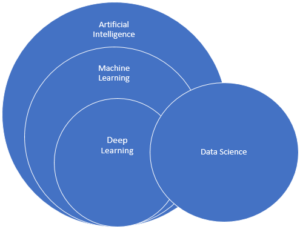
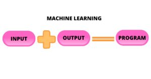
In simple words we can put this as: Machine Learning is a research field at the intersection of statistics, artificial intelligence, and computer science which gives the computer the ability to learn without being explicitly programmed, it can be defined as an automated process that extracts patterns (knowledge) from data. It is the science of about learning models that generalize well. In a way we can say that Machine Learning makes programming more scalable, as otherwise we all know that writing a software can be a very difficult task, thus with Machine Learning here, we do not have to burden ourselves with the manual process of programming, but instead we let the data do the work.

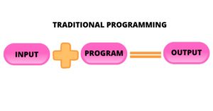
Traditional programming comprises of hand coded rules of “if” and “else” decisions to process data or adjust to user input and forming the logic to create the program, whereas Machine Learning is an automated process, the logic already exists, we must introduce right logic to right problem statement. Also, the approach of traditional programming language is limited, whereas machine learning models or algorithms has vast applications. For instance, face detection was an unsolved problem until as recently as 2001 Haar feature-based cascade classifiers a machine learning approach and other deep face recognition concepts came up.

“The human face is a dynamic object and has a high degree of variability in its appearance, which makes face detection a difficult problem in computer vision.”

— Face Detection: A Survey, 2001.

Below is the image of a standard Machine Learning Pipeline that includes the following steps, pipelining is the process of tying together different pieces of a machine learning process – creating a basic workflow of a standard machine learning model. The concept of pipelining is analogous to physical pipelining, but the term is highly misleading because the concept implies a one-way flow of data which is not the case in real.

• Collecting Data
• Analyzing Data
• Data Preparation or Data Wrangling
• Feature Extraction
• Training and testing the model
• Evaluating the model
• Prediction
• Feedback

“The goal is to turn data into information and information into insight.”

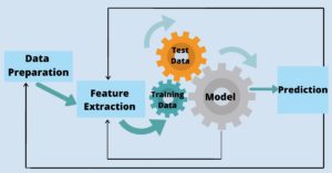
Standard Machine Learning Pipeline

Machine Learning is a subset of Artificial Intelligence and it can be broadly categorized to Supervised Learning, Unsupervised Learning and Reinforcement Learning.

Supervised Learning –

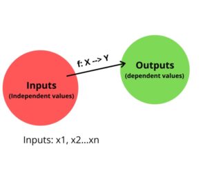
Indicates the presence of a supervisor as a teacher, the algorithm signifies learning a function that maps an input to an output based on example input-output pairs. Here, the algorithm based on inference from the labeled training data produces general hypotheses, which then makes predictions about future instances. Broadly speaking, Supervised Learning creates a function, or a model that maps the relation between the input variable and the output variable i.e. it helps us to analyze the relationship between the dependent and the independent variable/variables. The dependent variable is what we want to predict, and the Independent variable is what we use to predict the output. The supervision comes in the form of the wanted output, which in turn lets you adjust the function based on the actual output it produces.

Data is in the form of {xi, yi}, where i=1,2,3..n

x= Input data or feature vector

y= Output data

y= f(x), the mapping function

Supervised learning generates a function that maps inputs to desired outputs.

It allows you to train your system to make pricing predictions, adjustment campaign, customer recommendations, and much more, while allowing the system to self-adjust and make decisions on its own. Supervised learning can be further grouped into two broad categories – Regression and Classification.

Classification –

A classification problem is when the output variable is categorical or discrete value, such as identifying whether the person is male or female, or an e-mail is ‘spam’ and ‘not spam’. Speaking of which, classification is a technique where we categorize data into a given number of classes. A classification problem requires the outputs or samples to be classified into one of two or more classes i.e. a problem can be solved by Binary Classification or Multi class classification or Multi label classification, with the main goal of the classification problem being identification of the category/class to which a new data will fall under.

Classification Algorithms:

• Logistic Regression

• k-Nearest Neighbors

• Naïve Bayes

• Decision Tree

• Random Forest

• Support Vector Machine

  We shall discuss few of the algorithms in this blog.

Logistic Regression: Logistic regression is used for classification problems, it is a predictive analysis algorithm which is based on the concept of probability, and the prediction is based on the use of one or several predictors (Numerical and Categorical). It is used when the dependent variable (target) is categorical, i.e. it predicts the probability of an outcome that can only have two values (dichotomy). Below is the image of a Logistic regression derived from Linear regression function, signifying that a Logistic regression is an extension of a simple Linear regression. But logistic regression uses a more complex cost function termed as the ‘Sigmoid function’ instead of a linear function to transform its output and return a probability value.

                                                        Logistic Regression from Linear Regression

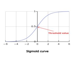
Sigmoid function has a characteristic ‘S’ shaped curve or sigmoid curve and is defined by:  y = 1/(1+e^(-z))

It is a type of activation function, and more specifically defined as a squashing function. Squashing functions limit the output to a range between 0 and 1, making these functions useful in the prediction of probabilities. The logistic function applies a sigmoid function to restrict the y value from a large scale to within the range 0–1.

Where, z = ß0 +ß1x which is similar to y = mx + c of linear regression.

Decision Bound

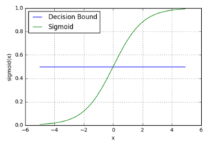
Image Source: ML Glossary

In the graph, the value 0.5 indicates the threshold value or the tipping value, the values equal to or above 0.5 is rounded off to 1 and the values below 0.5 is reduced to 0. With this the threshold value indicates the probability of 1 or 0 (i.e. binary format).

We can therefore make our predictions based on the sigmoid function and decision boundary. K-Nearest Neighbors: K Nearest Neighbors algorithm is a non-parametric, lazy learning algorithm that can be used to solve both classification and regression problems. The algorithm uses ‘feature similarity’ to classify new cases based on a similarity measure (e.g., distance functions). By non-parametric we mean that the no. of parameters is not fixed and can grow as it learns from more data. A non-parametric algorithm is computationally slower but makes fewer assumptions from the data.

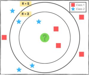
The Distance function can be Euclidean, Minkowski, Manhattan or Hamming, Euclidean, Minkowski and Manhattan function is used for continuous variables whereas Hamming is used for categorical variables.

Euclidean distance

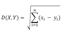
Minkowski distance

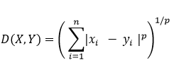
Manhattan distance

Hamming (or overlap metric) distance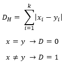

The most commonly used distance metric for continuous variables is Euclidean distance.

The choice of k depends upon the data, choosing the right value of k is a process called parameter tuning and is important for better accuracy. In general, larger values of k reduces effect of the noise on the classification but make boundaries between classes less distinct, whereas a small value of k means that noise will have a higher influence on the result and a large value make it computationally expensive. To be noted that k-NN is highly affected by outliers or noise therefore it is extremely important to carefully select or scale features to improve classification.

Regression –

Regression is a set of techniques for estimating relationships, between multiple variables. A regression problem is when the output variable is continuous/quantitative, such as ‘height’, ‘weight’, ‘dollar’.

It refers to the problem of learning the relationships between some (qualitative or quantitative) input variables x = [x1 x2 . . . xp] and a quantitative output variable y. In mathematical terms, regression is about learning a model y = ß0 + ß1 *x, where ß0 is a noise/error term which describes everything that cannot be captured by the model. With our statistical perspective, we consider ß0 to be a random variable that is independent of x and has a mean value of zero. There are several types of Regression techniques, these techniques are mostly driven by three metrics -number of independent variables, type of dependent variables and shape of regression line, for instance:

• Linear Regression

• Polynomial Regression

• Ridge Regression

• Lasso Regression

• Stepwise Regression

• ElasticNet Regression

Linear Regression: Linear Regression establishes a relationship between dependent variable (Y) and one or more independent variables (X) using a best fit straight line (also known as regression line). It is a simple approach to supervised learning. It assumes that the dependence of Y on x1, x2, . . . xp is linear. This linear approach can be related to the force for stretching a spring and the distance that the spring stretches (in Hooke’s law). Below is the image of a Linear Regression model, the red line indicates the best fit straight line while the blue dots indicate the data points.

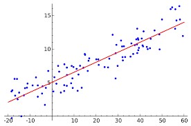
The Linear equation is represented by a simple equation as below:

Here, x is called the independent variable or predictor variable, and y is called the dependent variable or response variable.

• β1 is the slope of the line: this is one of the most important quantities in any linear *regression analysis. A value very close to 0 indicates little to no relationship; large positive or negative values indicate large positive or negative relationships, respectively. For our Hooke’s law example earlier, the slope is the spring constant
• β0 is the intercept of the line or bias

The Details:

Regression Analysis is a form of predictive modelling technique which analyzes the relationships between one independent and one dependent variable.

The cost function helps us to figure out the best possible value of β0 & β1 which would provide the best fit line for the data points, while the Gradient descent function is a method to update β0 & β1 thereby reducing the cost function.

Cost Function

Cost functions also referred to as the loss function, is used to estimate the errors in the performance of the model. Simply put, a cost function is a measure of how wrong the model is in terms of its ability to estimate the relationship between X and y. It is basically the difference between predicted value and actual value.

The fundamental objective is to minimize the cost function. Now comes the Gradient descent function is used to find a local minimum of a function is an efficient optimization algorithm that attempts to find the local or global minima of a function. It enables the model to learn the gradient or the direction to minimize the error. By direction we mean how the parameters are tuned to reduce the cost function, this method is tried iteratively until we reach the convergence, where further tweaks to the parameter produce little to zero changes in loss.

Gradient descent is also known as steepest descent.

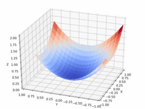
Gradient Descent

This is part 1 of the blog series, the next blog will be an extension of Machine Learning fundamentals covering unsupervised learning.